Data Analysis > Correlation and Regression > Chi-Square Test of Independence
Chi-Square Test of Independence (for categorical variables)
To create a contingency table
table(lung$sex,lung$ph.ecog)
tab <- table(lung$sex, lung$ph.ecog)
row_perc <- prop.table(tab, margin = 1) * 100
To find rounded to 1 decimal place of all percentages:
round(row_perc, 1)
chisq.test(tab)
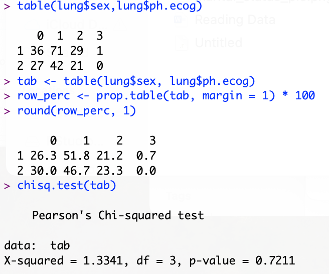
p-value much more greater than 0.05. so null hypothesis is rejected i.e. sex and performance score are not independent.
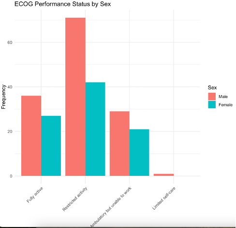
For a keen observation we can plot the grouped bar chart:
rownames(tab) <- c("Male", "Female")
colnames(tab) <- c( "0: Fully active",
"1: Restricted activity",
"2: Ambulatory but unable to work",
"3: Limited self-care")
barplot(tab,
main = "ECOG Performance Status by Sex",
xlab = "ECOG Status", ylab = "Frequency",
col = c("skyblue", "salmon"),
legend = rownames(tab), beside = TRUE, las = 2,
cex.names = 0.8) # scale x-axis label text

barplot(tab,
main = "ECOG Performance Status by Sex",
xlab = "ECOG Status", ylab = "Frequency",
col = c("skyblue", "salmon"), legend = rownames(tab),
beside = FALSE, las = 2,
cex.names = 0.8) # scale x-axis label text

library(ggplot2)
tab <- table(lung$sex, lung$ph.ecog)
rownames(tab) <- c("Male", "Female")
colnames(tab) <- c( "Fully active",
"Restricted activity",
"Ambulatory but unable to work",
"Limited self-care")
df <- as.data.frame(tab)
ggplot(df, aes(x = Var2, y = Freq, fill = Var1)) +
geom_bar(stat = "identity", position = "dodge") +
labs(title = "ECOG Performance Status by Sex",
x = "ECOG Status", y = "Frequency", fill = "Sex") +
theme_minimal() +
theme(axis.text.x = element_text(angle = 45, hjust = 1))
Correlation for ordinal variables
No More
Feedback
ABOUT
Statlearner
Statlearner STUDY
Statlearner